4.1: Areas and Distances

We are now in a position to talk about the integral.

First, let's discover what the formula for the integral depends on.

Before we do so, we need to discuss sigma notation.

Sigma Notation

Suppose you would like to add \[1 + 2 + 3 + 4 + 5 + \cdots + 100\] You can compactly represent this sum in sigma notation: \[1 + 2 + 3 + 4 + \cdots + 100 = \sum^{100}_{i = 1} i\]

The $i$ below the sigma is called the index.
$i$ is typically a natural number, and increases by 1 until it is equal to the number above the sigma.

Evaluate the following sums:

$\displaystyle \sum^{5}_{i = 1}(-1)^i\cdot i$
$\displaystyle \sum^{5}_{i = 1}i\cdot f(i)$ given that $f(x) = x$.

The Distance Problem

In calculus, the distance problem is finding the total distance traveled over a time period if you know the velocity at all time periods.

You are driving at 75 miles per hour. How far have you traveled after two hours?

This example shows two things:

From velocity, we found distance. Sounds like an antiderivative (we started with $f'(x)$ and found $f(x)$)!
The calculation utilized the area underneath the graph and between the $x$-axis.

The Area Problem

In calculus, the area problem is finding the area underneath the curve and between the $x$-axis for a given function.

The previous problem had straight lines. But this "area underneath the curve" also works for curved lines.

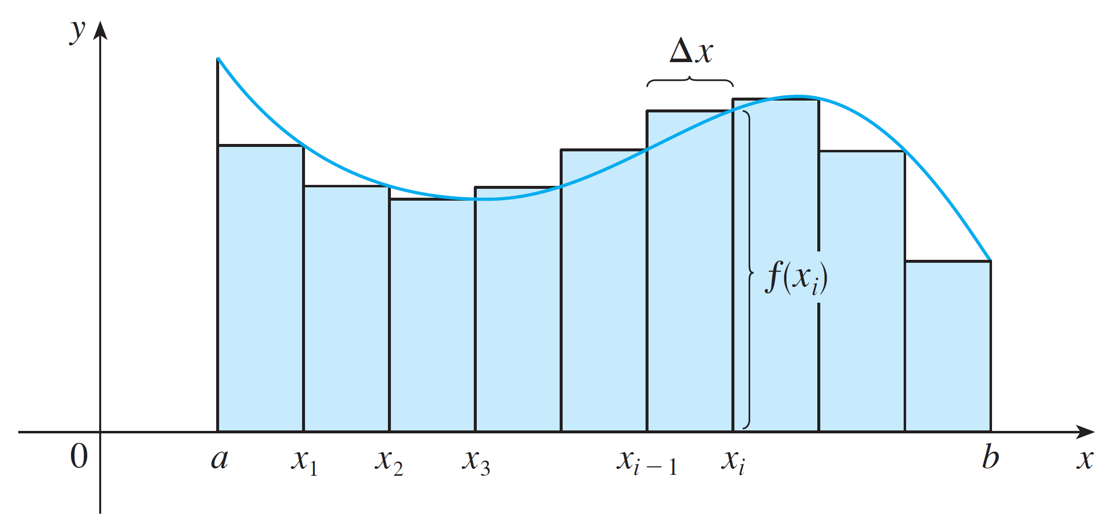
Step 1: Approximation With Rectangles

Estimate the area between the graph and the $x$-axis of the function \[f(x) = x^2, \ \ [0, 1]\] using four rectangles and right endpoints for rectangle height.

Estimate the area between the graph and the $x$-axis of the function \[f(x) = x^2, \ \ [0, 1]\] using four rectangles and left endpoints (for rectangle height).

Step 2: Use More Rectangles!

Here is the previous problem animated when using the left endpoints for the heights:

Notice how the approximation gets better and better as we use more and more rectangles.

Consider $n$ to be the number of rectangles. Then in our previous sum we need to incorporate $\displaystyle\lim_{n\rightarrow \infty}$!

For $f(x) = x^2$ on $[0, 1]$, use $n$ rectangles and right endpoints.

This limit of sums of rectangles gives the exact area underneath the curve.

In our example, the exact area underneath the curve of $f(x) = x^2$ on $[0, 1]$ is the expression \[\lim_{n\rightarrow \infty} \dfrac{1}{n^3} \sum^n_{i = 1} i^2\]

In general

The area that lies underneath the graph of the function $f(x)$ on the interval $[a, b]$ is the limit of the sum of the approximating rectangles: \begin{align} A &= \lim_{n\rightarrow \infty} \left[f(x_1)\Delta x + f(x_2)\Delta x + \cdots + f(x_n) \Delta x\right] \\&= \lim_{n\rightarrow \infty} \sum^n_{i = 1}f(x_i)\Delta x \end{align} where

$\Delta x$ is the width of one rectangle, or $\Delta x = \dfrac{b - a}{n}$
$x_i$ is the right endpoint of the $i$th rectangle, where $x_i = a + i\cdot\Delta x$

This limit sum formula is called the definite integral. See the next section.