3.4: Marginal Functions in Economics

Cost Functions

---

Let's first define what marginal means.

Marginal cost is the cost incurred when producing one additional unit given that you are already at a certain level of operation.

The number given in part (a) is a marginal cost.

Part (c) showed the derivative evaluated at the certain level of operation is close to the marginal cost.

This reason is why economists have defined the marginal cost function to be the derivative of the cost function.

Average Cost Functions

---

Instead of looking at the total cost incurred at level $x = a$, we can look at the average cost per unit incurred at level $x = a$.

Naturally, $\bar{C}'(x)$ is the marginal average cost function.

Not all average cost functions with behave in such a manner.

We will now define the marginals for revenue and profit function.

Revenue and Profit Functions

Let's first define what demand is.

The revenue function $R(x)$ gives you the total revenue realized from the sale of $x$ units. $R(x)$ can be thought of in the following way: if a company charges $p$ dollars per unit, then \[R(x) = px\]

The unit selling price $p$ is affected by demand, among other variables. If we simplify our mathematical model of price and ignore the other variables, then by definition \[p = f(x)\] and substituting into $R(x)$ we see that \[R(x) = px = x\cdot f(x)\]

Similar to the initial example in this section, the marginal revenue gives the revenue realized when another unit is sold given that sales are already at a certain level. By a similar argument (derivative close to marginal), we define the marginal revenue function as $R'(x)$.

We also define the marginal profit function as $P'(x)$. It is an approximation of the actual profit realized from the sale of the $(x+1)$th unit, assuming the $x$th unit sold.

Elasticity of Demand

---

Let's use the concepts in this section to analyze the demand function.

Recall that the demand function follows the equation $p = f(x)$. For example, \[p = -0.025(x+10)^2 - 0.5(x+10) + 60\]

If we solve for the quantity $x$ in that equation instead (not always possible), our demand function is $x = f(p)$, meaning plugging in price gives the total quantity demanded.

Be careful! The axes are switched now.

Here is an example of such a function:

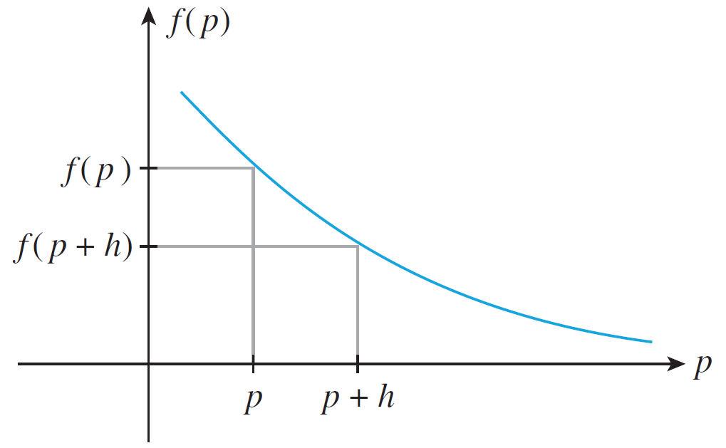
Let's think about a certain price $p$.

If $p$ is increased from $p$ to $p+h$ dollars, then the quantity demanded is predicted to drop from $f(p)$ to $f(p+h)$ units.

The percentage change in the unit price is \[\dfrac{h}{p}\cdot 100 \qquad \qquad \text{think} \qquad \dfrac{\text{change in unit price}}{\text{current price}}\cdot 100\]

The percentage change in the quantity demanded is \[\dfrac{f(p + h) - f(p)}{f(p)}\cdot 100 \qquad \qquad \text{think} \qquad \dfrac{\text{change in quantity demanded}}{\text{quantity demanded at price }p}\cdot 100\]

Let's take the ratio of these quantities. We have \begin{align} \dfrac{\text{percent change in quantity demanded}}{\text{percent change in unit price}} &= \dfrac{\frac{f(p + h) - f(p)}{f(p)}\cdot 100}{\frac{h}{p}\cdot 100} \\&= \dfrac{f(p + h) - f(p)}{f(p)}\cdot \dfrac{p}{h} \\&= \dfrac{f(p + h) - f(p)}{h}\cdot \dfrac{p}{f(p)} \end{align} If $f(x)$ is differentiable at $p$ and $h$ is small, then \[\dfrac{f(p + h) - f(p)}{h}\approx f'(p)\] so the aforementioned ratio is approximately equal to \[\dfrac{f'(p)}{\frac{f(p)}{p}} \approx \dfrac{pf'(p)}{f(p)}\]

The negative of this quantity is called elasticity of demand.

Elasticity and Revenue

---

Elasticity helps us analyze how revenue changes with respect to changes in unit price.

Recall that if $p = f(x)$, then $R(x) = px = xf(x)$.

In our formulation, we have $x = f(p)$, so we can rewrite \[R(p) = px = pf(p)\]

Now taking the derivative with respect to $p$: \begin{align} R'(p)= \dfrac{d}{dp}R(p) &= 1\cdot f(p) + pf'(p) \\&= 1\cdot f(p) + \dfrac{f(p)}{f(p)}pf'(p) \\&= f(p)\left[1 + \dfrac{pf'(p)}{f(p)}\right] \\&= f(p)[1 - E(p)] \end{align}

Consider when demand is elastic when the unit price is set at $a$ dollars. Then $E(a) > 1$, so $1 - E(a) < 0$.

Because $f(a)$ can never be negative (quantity demanded cannot be negative), the above equation becomes \[R'(a) = f(a)[1 - E(a)] = + \cdot - < 0\]

This means when demand is elastic at $p = a$, the revenue function $R(p)$ is decreasing at $p = a$.

In other words, a small unit increase in the unit price results in a decrease of the revenue.